We will look at in this blog, one of Gauss' \(8\) proofs of this. The proof by so called Gauss sums. This is a common proof presented in many elementary number theory class. but usually without any intuition: its just computation. We will assume some Field theory and Galois theory, basically just know the Galois correspondence. Also for our intents and purposes, \(2\) doesn't exist!

When is -3 a quadratic residue?

We start of with a simple question, when is \(-3\) a quadratic residue? So we are asking, let \(p\) be prime, does there exist \(x\) such that \[x^2 = -3 \pmod{p}?\] To do this, we will do a trick. Often you can figure out something for \(\mathbb{F}_p\) by thinking about it in \(\mathbb{C}\) first, or vice versa. An example of this is proving \(\mathbb{F}_p\) has cyclic multiplicative group by counting elements of order \(p\) in \(\mathbb{C}^\times\). Consider \(\omega\) to be a third root of unity, say \[ \omega = \dfrac{-1+\sqrt{-3}}{2}.\] Notice that you can hence write \(\sqrt{-3}\) interms of third roots of unity, lets say \(\sqrt{-3} = \omega-\omega^2\). So if I have the analogue of a third root of unity in \(\mathbb{F}_p\), then i expect \(-3\) to be a square root. Well there is an element of order \(3\) if and only if \(3|p-1\), i.e if \(p\equiv 1 \pmod{3}\).

Let \(p\equiv 1 \pmod{3}\), and \(z\) an element of order \(3\) in \(\mathbb{F}_p\). Then we claim, motivated by the complex case, that \((z-z^2)^2 = -3\). Indeed, this is a simple computation: \[ (z-z^2)^2 = z^2-2z^3+z^4 = z^2-2+z = (z^2+z+1)-3 = -3.\] So actually we just proved that if \(p\equiv 1\pmod{3}\), then \(-3\) is a quadratic residue mod \(p\).

What about when \(p\equiv 2 \pmod{3}\)? We do not have an element of order \(3\) so we cannot do this nice trick. But what we can do is adjoint an element of order 3, i.e look at \(\mathbb{F}_p[z]\) where \(z\) is a root of \(z^2+z+1=0\). In this case, we also have \((z-z^2)^2 = -3\). Since this is a field, the equation \(x^2=-3\) can only have two solutions, i.e \(z-z^2\) and its negative. So the question now: is \(z-z^2\) actually in the basefield \(\mathbb{F}_p\)? Here we will use some light Galois theory: notice \(z\mapsto z^2\) is an automorphism but doesnt fix \(z-z^2\). This means \(z-z^2\) isnt in the base field, i.e \(-3\) has no square root.

The trick we did for \(p\equiv 2\pmod{3}\) will not generalize unfortunately. The reason is that we do not easily know what the minimum polynomial of \(z\), an element of order \(q\), is in \(\mathbb{F}_p\). So we do not know which \(z\mapsto z^a\) are the correct automorphisms to consider! However, once we look at the general case, actually an even nicer trick will help us.

Gauss sums

We managed to completely classify when \(-3\) is a quadratic residue mod \(p\) by writing its square root interms of roots of unity. We will try to ask a more general question, when is \(\sqrt{n}\in \mathbb{Q}(\zeta_p)\) where \(\zeta_p\) is a primitive \(p\)th root of unity. Is there even such an element in the field? Actually the answer is yes. To see this all we need is some Galois theory. Note \[\Gal(\mathbb{Q}(\zeta_p)/\mathbb{Q}) = \{\sigma_j| j \text{ coprime to } p\} \cong \left(\mathbb{Z}/p\mathbb{Z}\right)^\ast \cong \mathbb{Z}/(p-1)\mathbb{Z}, \quad \sigma^j(\zeta_p) = \zeta_p^j. \] And since \(2\) isnt a prime, this is an even cyclic group and hence has a subgroup of index \(2\). The fixed field of this is hence of degree 2, i.e a quadratic extension \(\mathbb{Q}(\sqrt{n})\) so in particular, some square root is in the cyclotomic field. Note the subgroup of index \(2\) will be all things of the form \(\{\sigma_{j^2}\}\).

But lets not get too lost in the Galois theory, and lets say simply that we have \[\tau = \sum_{i=0}^{p-1} a_i \zeta_p^i = \sqrt{n}\] for some \(n\). Then since an automorphism sends \(\sqrt{n}\) to one of its conjugates, i.e itself or its negation, we would have \(\sigma_j(\tau) =\pm \tau\). But in either case, we could just apply \(\sigma_j\) again to have \(\sigma_{j^2} (\tau) = \tau\). If we expand this out, it says \[\sigma_{j^2}(\tau) = \sum_{i=0}^{p-1} a_i \zeta_p^{j^2i} = \tau = \sum_{i=0}^{p-1} a_i \zeta_p^i.\] Comparing the coefficient of \(\zeta_p^{j^2}\), we have \(a_1 = a_{j^2}\). So this tells us that all quadratic residues have the same coefficient. Since \(\tau\) isnt fixed by everything, for non-residues we should have \(\sigma_{j}(\tau) = -\tau\), i.e \(a_j=-a_1\) and \(a_0=0\). We can just divide by \(a_1\) and hence we can assume \(a_1=1\). So the coefficient of \(\zeta^j\) is +1 or -1 depending on wether it is a quadratic residue or not. I.e \[\tau = \sum_{i=1}^{p-1}\left(\dfrac{i}{p}\right) \zeta_p^i.\] Now we compute \[\begin{aligned} \tau^2 &= \sum_{(i,i')\in \mathbb{F}_p^2} \left(\dfrac{ii'}{p}\right) \zeta_p^{i+i'} \\ &= \sum_{(i,k)\in \mathbb{F}_p^2} \left(\dfrac{i(ki)}{p}\right) \zeta_p^{i+ki}\\ &= \sum_{(i,k)\in \mathbb{F}_p^2} \left(\dfrac{k}{p}\right) \zeta_p^{i(k+1))}\\ &= \sum_{k\in \mathbb{F}_p} \left(\dfrac{k}{p}\right) \sum_{i \in \mathbb{F}_p} \zeta_p^{i(k+1)}\\ &= (p-1)\left(\dfrac{-1}{p}\right) + \sum_{k\in \mathbb{F}_p-\{-1\}} \left(\dfrac{k}{p}\right) \sum_{s \in \mathbb{F}_p} \zeta_p^{s}\\ &= (p-1)\left(\dfrac{-1}{p}\right) + \sum_{k\in \mathbb{F}_p-\{-1\}} \left(\dfrac{k}{p}\right)(-1)\\ &= p\left(\dfrac{-1}{p}\right) -\sum_{k\in \mathbb{F}_p} \left(\dfrac{k}{p}\right)\\ &= p\left(\dfrac{-1}{p}\right). \end{aligned} \] We used several time that whenever \(i\neq 0\), we have \(k\mapsto ki\) is a bijetion of \(\mathbb{F}_p^\times\). We already knew \(\tau^2\) was going to be a rational, so its great to see it is actually just \(\pm p\). Ofcourse when \(p=3\), this is the case we already worked out. Also recall that \(\tau\) is fixed by \(\sigma_q\) only when \(q\) is a quadratic residue mod \(p\). So \[\sigma_q(\tau) = \sum_{i=1}^{p-1}\left(\dfrac{i}{p}\right) \zeta_p^{qi} = \left(\dfrac{q}{p}\right) \tau.\] Unfortunately there is no nice way to finish this off in \(\mathbb{C}\), so we move down to finite fields as we did for \(p=3\).

Now consider \(\mathbb{F}_q\), and the question is wether \(p\) is a quadratic residue mod \(q\). Again, consider an extension \(\mathbb{F}_q(z)\), so we have an element of order \(p\). We know \[\tau = \sum_{i=1}^{p-1}\left(\dfrac{i}{p}\right) z^i\implies \tau^2 = p\left(\dfrac{-1}{p}\right).\] The computation would be the same but also one might argue using polynomials, the min poly of \(\zeta_p\) in \(\mathbb{C}\) is \(\Phi_p\) and it must divide \(\tau^2-p\), and the min poly of \(z\) mod \(q\) divides \(\Phi_p\). Note that if we define \(\sigma_q\) the same way as before, sending \(z\mapsto z^q\), its not necessarily an automorphism but it does still satisfy \(\sigma_q(z) = \left(\dfrac{q}{p}\right) \tau.\). Since \((a+b)^q = a^q+b^q\) in this field, we have \[\tau^q = \sigma_q(\tau) = \left(\dfrac{q}{p}\right) \tau.\] As we know \(\tau \in \mathbb{F}_q\) if and only if \(\tau^q = \tau\). So actually we already know the answer, \(p\left(\dfrac{-1}{p}\right)\) is a quadratic residue mod \(q\) iff \(q\) is a quadratic residue mod \(p\). We have already accomplished our goal, we know how to relate \(p\) being a quadratic residue mod \(q\) to the other way around. But lets write an equation down with this and say \[\tau^q = \tau (\tau^2)^{(q-1)/2} = \tau \left(\dfrac{-1}{p}\right)^{(q-1)/2} p^{(q-1)/2} = \left(\dfrac{-1}{p}\right)\left(\dfrac{-1}{q}\right)\left(\dfrac{p}{q}\right)\tau.\] Equating we'd have \[\left(\dfrac{-1}{p}\right)\left(\dfrac{-1}{q}\right)\left(\dfrac{p}{q}\right) = \left(\dfrac{q}{p}\right),\] which we can write nicely as \[\left(\dfrac{-1}{p}\right)\left(\dfrac{-1}{q}\right)=\left(\dfrac{p}{q}\right) \left(\dfrac{q}{p}\right).\]

conclusion

Hopefully this injected some intuition into the idea of the Gauss sums. Basically, Gauss sums are a way to capture quadratic Kronecker-Weber, that we can write every \(\sqrt{n}\) interms of roots of unities. And this was enough to solve quadratic reciprocity. This idea can be generalized to higher reciprocity laws also. Infact the full statement of Kronecker-Weber says that every abelian extension(i.e Galois group over \(\mathbb{Q}\) is abelian) is a subfield of a cyclotomic extension. And basically this allows one to write down all such higher reciprocity laws. This is the content of Class field theory.

The Gelfand Isomorphism

Recall a Banach space is a normed \(\bb{C}\)-vector space complete under the induced metric. A Banach algebra in turn is a Banach space with a multiplication, such that \(\norm{ab}\leq \norm{a}\norm{b}\). The simplest such objects to study are the abelian Banach algebras. For each unital abelian Banach algebra \(A\), take \(\Spec(A)\) to be the space of characters, i.e homomorphisms \(A\lra{\gamma}\bb{C}\). We can give \(\Spec(A)\) the weak*-topology and its easy to check due after applying the Banach-Alaoglu theorem that this is infact a compact space. Now we get a representation \[\Gamma: A \lra{} C(\Spec(A)),\quad \Gamma(a)(\gamma) = \gamma(a)\] The norm on \(C(X)\) for compact haussdorf \(X\), the space of continous functions \(X\lra{}\bb{C}\), is \(\norm{f}_\infty= \mathrm{sup}_{x\in X} |f(x)|\). We call this the Gelfand representation. Note we could have asked for \(A\) to be non-unital, and then the character space would have been locally compact haussdorf. We would have to use \(C_0(\Spec(A))\) then, the space of continous functions like before but they go to zero at infinity (think about infinity by thinking about the one point compactification.).

A \(C^\ast\) algebra is an algebra with an involution \(\ast\) such that \(\norm{a^\ast a} = \norm{a}^2\). Note that if pointwise complex conjugation is the involution, both \(C(Y)\) and \(C_0(X)\) are \(C^\ast\)-algebras.Now the big theorem due to Gelfand is that for commutative \(C^\ast\) algebras, the Gelfand representation is an isomorphism. This tells us each non-unital commutative \(C^\ast\)-algebra is dual to some LCH space, and that every unital commutative is dual to some compact haussdorf space. A lot of \(C^\ast\) theory now is to see how much of this isomorphism theorem we can translate over to the non-commutative case. So in a sense \(C^\ast\)-algebra is the study of non-commutative topology. With that being said, we expect concepts in topology to carry over to \(C^\ast\)-algebras and vice versa. We will see that for compactification today.

I should mention that this really is an (anti-)equivalence of categories between commutative \(C^\ast\) algebras and the category of LCH spaces with continuous maps. Send a space to its \(C_0\) and a commutative algebra to its spectrum.

Unitizations and Compactifications

We shall say compact \(Y\) is a compactification of LCH \(X\) (non-compact) if

The easiest example of this is \(\opc{X}\), the one point compactification. This is just adding a single point to \(X\), call it \(\infty\), to make it compact. We can also write it by its universal property, that any compactification of \(X\) maps into \(\opc{X}\), i.e \(\opc{X}\) is the "smallest" compactificaiton.

As mentioned before, the philosophy is that every topological concept should have an analogue in operator theory. So lets look at \(C(\opc{X})\) towards that end. Notice that we have a map \(C(\opc{X})\lra{\cong} C_0(X) \oplus \bb{C}\) sending \(f\mapsto ((f-f(\infty))\mid_{X},f(\infty))\). It is easy to see this is an isomorphism. So adjoining a unit like this is the analogue of the one-point compactification. Lets try to find the analogues for compactifications in general. There is a unique norm on each \(C^\ast\)-algebra that satisfies the \(C^\ast\) identity, I leave it as an exercise to figure out the norm on \(C_0(X)\oplus \bb{C}\) making it a \(C^\ast\)-algebra.

Let \(X\lra{\iota}Y\) be a compactification of \(X\). Consider \(f\in C_0(X)\), then it extends to a \(\opc{f} \in C(\opc{X})\). We can combine the map \(Y\lra{}\opc{X}\) given by the universal property of \(\opc{X}\) and \(\opc{f}\) to get an element of \(C(Y)\).

A unitization of a \(C^\ast\)-algebra \(A\) is:

I have already shown compactifications lead to unitizations.I leave it as an exercise to show the converse.

Multiplier Algebras.

The Stone-Čech compactification of a LCH space \(X\), \(\beta X\), is the biggest compactification of \(X\). As we saw above, we expect this to correspond to the biggest unitization of a non-unital \(C^\ast\)-algebra \(A\). The advantage of thinking in these terms is that for \(C^\ast\) algebras this is quite explicit. Indeed, the biggest unitization of \(A\), called \(M(A)\)(its multiplier algebra) is given as follows:

\(M(A)\) is the set of double centralizers \((L,R)\) on \(A\). This means:

Suppose \(B\) contains \(A\) as an ideal. Then notice we have a map \(\psi:B\lra{}M(A)\), by sending \(c\mapsto (L_c,R_c)\) again and using the fact that \(A\) is an ideal. This extends the cannonical map \(A\lra{} M(A)\). This is infact unique, for say \(\phi:B\lra{} M(A)\) also extended it. Then for \(b\in B, a\in A\), we would have \[\psi(b) (L_a,R_a) = \psi(ba) = (L_{ba},R_{ba}) =\phi(ba) = \phi(b) (L_a,R_a)\] So that \( (\phi(a)-\psi(a)) A =0\) in \(M(A)\), but \(A\) is essential in \(M(A)\) so \(\phi(a)=\psi(a)\). Finally suppose \(A\) is essential in \(B\), then if \(b\in \ker(\psi)\) then \(L_b(A) = bA=0\), so that \(b=0\). Hence the map is injective.

To summarize, whenever \(B\) contains \(A\) as an essential ideal, \(B\) has a unique embedding into \(M(A)\). So \(M(A)\) is the biggest unitization as promised. We will get to the commutative case in the next section, but a good example for now is that if \(A=K(H)\), compact operators on some hilbert space, then \(M(A) = B(H)\), bounded operators on that hilbert space.

Stone-Čech Compactification

The Stone-Čech Compactification, \(\beta X\),is the biggest compactification of a space, i.e if \(Y\) is a compactification than \(\beta X\) uniquely maps into \(Y\) making the obvious diagram commute. This is literally the dual condition of the multiplier algebra, so we just need to figure out what \(M(C_0(X))\) is. Luckily for us, the answer is easy: \(C_b(X)\), bounded continuous functions on \(X\) with sup norm. One can easily check that \(C_0(X)\) is essential in \(C_b(X)\), so that there is a injective map \(\psi: C_b(X) \lra{} M(C_0(X))\). All we need to do is show surjection, which is easily done but the proof I know is a bit annoying and uses some other tools (like approximate units). I will hence refer the user to Gerard Murphy's book on the topic, page 83.

By the Gelfand Isomorphism, we know that \(C_b(X)\cong C(\beta X)\) for some \(\beta X\), and by the universal property discussed before, this \(\beta X\) is indeed the Stone-Čech compactification of \(X\). This proves that such a compactification exists in the first place but also gives a very nice explicit form for what the space should be.

Galois theory of covering spaces

First, we are going to develop the Galois theory for covering spaces. Covering spaces of \( X\) are maps \( p:Y\longrightarrow X\) such that around each point \( x\in X\) there is a neighborhood \( V\ni x\) such that \( p^{-1}(V)= \coprod U_i\) with the restrictions \( p: U_i\longrightarrow V\) is a homeomorphism. That is to say that there lies over this neighborhood in \(X\) disjoint copies of it in \(Y\) . The classic example of a covering space is the real number line covering the circle: the map \(\mathbb{R}\longrightarrow S^1\) defined by sending \(x\mapsto e^{2\pi i x}\) . This is demonstrated in figure 1.

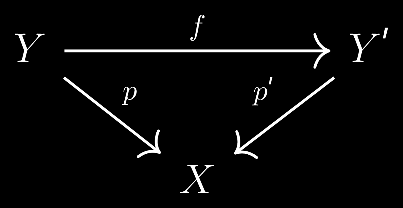
Now morphisms of covering spaces are as shown in the diagram below, defined this way as we care about the things that lie above a point and these preserve that. And then by \(\text{Aut}(Y|X)\) we will mean the automorphisms of \(Y\) as a covering space for \(X\) . By subcovers of \(p:Y\longrightarrow X\) we will mean covers \(p':Y'\longrightarrow X\) such that there is a morphism of covers \(f:Y\longrightarrow Y'\) which is also a covering map of \(Y'\) .Now for nice spaces (path connected,locally path connected and semi-locally simply connected spaces) there is a maximal connected cover (i.e every connected cover of \(X\) is covered by this). We call this the universal covering \(\tilde{X}\) of \(X\) .As an example the universal cover of the circle is the real number line. It turns out that this space is simply connected, and that \(\text{Aut}(\tilde{X}|X)\cong \pi_1(X)\) . The idea is that \(\pi_1(X)\) are all the loops in \(X\) , and if you lift the loop along a covering map, you get a path in \(\tilde{X}\) . Then take all the preimages of a point and lift a loop with the begining being a set point in the preimage, and then look at the endpoint of the lifted path.There is a unique automorphism that permutes the preimages like this(from begining of path to the end). The maximality of the universal cover would ensure that this map \(\pi_1(X,x) \longrightarrow \text{Aut}(Y|X)\) we just described by lifting loops is an isomorphism. For example lifting paths from the circle is like translation in the real number line, which would corrospond to the winding number of a circle. For all the details on why an universal cover exists and how to find its automorphism group, I refer the reader to chapter 1 of Hatcher's "algebraic topology".

Now, it is clear that \(\text{Aut}(Y|X)\) acts on the fibres of a given point. This is much like how the galois group of a field extension acts on the set of roots of a polynomial. Now we like this extension when its a Galois extension, i.e the galois group acts transitively on the roots of a polynomial and the extension is seperable (latter is irrelevant to our case). So a natural way to define a galois covering is to require this deck action of \(\text{Aut}(Y|X)\) on the preimages of \(x\) to be transitive. Does this yield good theory? the answer is yes. Note that in particular the universal cover is a galois cover.

Suppose \(p:Y\longrightarrow X\) is a galois cover, then subgroups of \(\text{Aut}(Y|X)\) corrospond to subcovers of \(Y\) and normal subgroups to galois subcovers. The corrospondence is defined as follows: for a subcover \(Y'\) simply send it to the subgroup \(\text{Aut}(Y|Y')\) and for a subgroup \(H\) send it to the orbit space of \(Y\) with respect to the action of \(H\) (topologized with the quotient topology, this will be a subcover.). Notice that this is almost completely analogous to vanilla galois theory for fields. We send a subfield to a galois group and we send a subgroup to its fixed subfield. We also have, similar to vanilla Galois theory that \(\text{Aut}(Y'|X) \cong \text{Aut}(Y|X)/\text{Aut}(Y'|X)\) . I will leave proving all of this as an exercise for the reader.

Riemann surfaces and their function fields

A riemann surface is a topological space \(X\), together with a collection of charts (called an atlas)\(\phi_i:U_i \longrightarrow V_i\) where \(U_i\) is an open subset of \(X\) and \(V_i\) an open subset of \(\mathbb{C}\) with \(\phi_i\) being a homeomorphism. This is to say that our space locally looks like the complex plane. We require the addition condition that for two charts \(\phi_i\) and \(\phi_j\) we should be able to transition holomorphically. That is to say \(\phi_i\phi_j^{-1}\) is a holomorphic map (which makes sense as this is a map between subsets of \(\mathbb{C}\). This condition exists to allow us to define holomorphic maps of riemann surfaces, I.e say a map \(f:X\longrightarrow \mathbb{C}\) is holomorphic if for each point has a chart with \(f\phi_i^{-1}\) is holomorphic. The transition maps being holomorphic means that if we had another chart around a point, we could simply transition to a chosen one holomorphically and this property would be preserved. We can similarly define a holomorphic map between two surfaces \(f:X\longrightarrow Y\) to be a map such that \(\phi_{yj} f \phi_{xi}^{-1}\) is always holomorphic. So we have essentially defined these surfaces that we can do complex analysis on. Now we say that two atlases on \(X\) are compatible if their union is also an atlas (i.e you can holomorphically tansition between the two atlases). Because of this when we talk about a Riemann surfaces, we just assume it has a maximal atlas on it.

Now as examples of Riemann surfaces, we have the complex plane, with a single chart just being the identity map. We also have the Riemann sphere \(\mathbb{CP}^1\) which topologically is the same as a 2-sphere. We make it a riemann surface by considering this as \(\mathbb{C}\cup \{\infty\}\) (we get this by stereographic projection, draw the sphere in 3d and take the xy plane. Then draw a line through the northpole and a selected point and see where it intersects the plane. Everything except the north pole gets mapped to the plane, and the northpole under this would in a sense "get mapped to infinity".), and then giving it two charts. one of them is simply the identity on the open subset \(\mathbb{C}\), and the other is the map \(z\mapsto \dfrac{1}{z}\) on everything but \(0\).

Now we can define meromorphic functions on a surface in the same way as holomorphic functions,i.e functions so that \(f\phi^{-1}\) is meromorphic for all charts(so they are holomorphic if you remove a discrete set called the poles.) Notice that the holomorphic functions on \(X\), \(\mathscr{O}(X)\) is a ring under function addition and multiplication. Now the Meromorphic functions \(\mathscr{M}(X)\) actually go a bit further, they form a field, as they are allowed to take on the value of infinity. Also notice that if we have a holomorphic map \(f:Y\longrightarrow X\), then we have an induced \(f^\star:\mathscr{M}(X) \longrightarrow \mathscr{M}(Y)\) defined by sending the meromorphic function \(h:X\longrightarrow \mathbb{CP}^1\) to \(hf:Y\longrightarrow \mathbb{CP}^1\). Now field homomorphisms are always injective, so this actually induces a field extension of \(\mathscr{M}(X)\).

Now we do a computation, for \(\mathscr{M}(\mathbb{CP}^1)\). Now since the Riemann sphere is compact, there are only finitely many poles for a meromorphic function (as the poles form a discrete set). So we can multiply by appropriate factors to get rid of the poles on the \(\mathbb{C}\) part, for example multiplying by \((x-1)^2\) would get rid of a pole of order \(2\) at \(x=1\). Now this meromorphic function restricted to the complex plane is holomorphic, and hence a power series. Notice that the power series now has to terminate, as otherwise the pole at infinity would not be finite. So this is really a polynomial, and since we multiplied by another polynomial to get to this form, our meromorphic function is a rational function. So \(\mathscr{M}(\mathbb{CP}^1)=\mathbb{C}(t)\). So to study field extensions of this field, we should study holomorphic maps into the Riemann sphere.

</section>

Holomorphic maps of compact surfaces are branched covering maps

If we have a map between Riemann surface, it locally looks like \(z\mapsto z^k\) for some k, the ramification index of \(z\).What this means is that for each holomorphic map \(f:Y\longrightarrow X\) and each point \(z\in Y\), we can find charts such that \(\psi f\phi^{-1}=z^k\). I refer the reader to Forster's "lecture on Riemann surfaces" theorem 2.1 for the proof.This implies the open mapping theorem, that holomorphic maps send open sets to open sets. Now notice that whenever \(k=1\) we have a local homeomorphism around that point, as \(f\) would be injective and open mapping theorem means the local inverse would be too.

Now suppose we have a map \(f:Y\longrightarrow X\) is of compact riemann surfaces. Now consider the set of unramified points (points with \(k\geq 2\)) \(A\), then \(A\) is discrete. This is because the map locally looks like \(z^k\) and we can always take a small neighborhood not containing \(0\) on which this is a local homeomorphism. So we have a finite number of unramified points for maps between compact surfaces. Now the open mapping theorem gives us that whenever \(X\) is connected, \(f\) is surjective. This is because the image of \(Y\) would be both open and compact(and hence closed), and connected spaces only have trivial clopen sets. So now for each unramified point \(x\in X\), let \(y_i\) be the preimages, and then pick a neighborhood \(U\ni x\) and neighborhoods \(V_i\ni y_i\) with \(f:V_i \longrightarrow U\) a homeomorphism (we can do this because local homeomorphism). We can pick the \(V_i\) to be all disjoint and then \(f^{-1}(U)=\cup_i V_i\). So if we remove the ramified points we actually have a covering map.

We showed that holomorphic maps between compact surfaces are branched coverings, now we show the converse. If \(X\) is a Riemann surface, and \(f:Y\longrightarrow X\) a covering map, then we can pull back the charts on X onto Y (i.e \(\phi_i f\) on Y are the charts) and then by construction this makes \(f\) into a holomorphic map. So now we have a direct analogy between the two galois theories, we have the galois theory of coverings from holomorphic maps(as these are almost covering maps) and the field extension of the meromorphic fields induced by these maps.

The covering Automorphism group is the same as the Galois group

Lets say we have a covering map \(f':Y'\longrightarrow X'\) where \(X'\) is \(X\) with a finite set of (unramified) points removed, we can uniquely extend this to a branched cover (and hence a holomorphic map) of \(X\). See Forster theorem 8.4 for proof, and then theorem 8.5 to see that covering morphisms of \(Y'\) and \(Z'\) over \(X'\) extend uniquely to that of holomorphic maps between \(Y\) and \(Z\) (these are the unique spaces where the covering maps extend to) over \(X\). Notice the latter means each morphism of \(Y'\) to \(Z'\) induces a field homomorphism from \(\mathscr{M}(Z)\)to \()\mathscr{M}(Y)\) that fixed \(\mathscr{M}(X)\). In particular we have a morphism \(\text{Aut}(Y'|X')\longrightarrow \text{Gal}(Y|X)\). Now if the covering is galois then this is injective as different holomorphic maps induce different field automorphims. Now if the galois covering was of degree n, then its automorphism group is of order n(how one point is sent to another uniquely determines a cover automorphism). To show surjectivity, we want to show that the galois groups for the field extension also has order n.

So first suppose we have a meromorphic function \(h\in\mathscr{M}(Y)\). Take a point \(x\in X'\) and a neighborhood \(U\ni x\) with \(f^{-1}(U) = \cup V_i\), with the \(V_i\) disjoint, so that \(f: V_i\longrightarrow U\) are homeomorphisms. Now call the inverse \(s_i:U\longrightarrow V_i\), and \(h_i = h s_i\) meromorphic functions on \(U\). Now take the symmetric polynomials \(a_k\) in the \(h_i\), and \(\prod(t-h_i)\) which has the symmetric polynomials as coefficients, then these are also meromorphic functions on \(U\). Now if we do this for all points \(x\in X'\) and glue the symmetric polynomials together (as on intersection of two such open sets they have to agree) we get global functions \(a_k\) on \(X\), and hence a Global polynomial with the coefficients \(a_k\). Now \(h\) satisfies this polynomial as its restriction to one of these \(U\)s is \(\prod(h-h_if)=0\), and then we glue it together to get its \(0\) globally on \(Y'\). Note that we used \(h_i f\) as the field extension is really \(\mathscr{M}(Y)|f^\star \mathscr{M}(X)\). This means all meromorphic functions on Y satisfy an irreducible polynomial of degree less than n over \(f^\star\mathscr{M}(X)\). Finally we use Riemann's existence theorem, which garuntees a function \(h\in\mathscr{M}(Y)\) which would seperate the \(y_i\) lying over a given \(x\),which means that the polynomial has to have degree n. For proof of Riemann's existence theorem, I refer the reader to Forster's chapter 2 which uses sheaf cohomology to prove it. Now \(\mathscr{M}(X)(h) = \mathscr{M}(Y)\). This is because if we had another \(g\in \mathscr{M}(Y)\) then \(\mathscr{M}(X)(h)\subset \mathscr{M}(X)(h,g)= \mathscr{M}(X)(k) \) by primitive element theorem, and since \(k\) has degree atmost n, we have the equality \(\mathscr{M}(X)(h) = \mathscr{M}(X)(k)\) and so \(g\in \mathscr{M}(X)(h)). This proves the galois group has order n and hence that the covering automorphism group is the same thing as the galois group.

Combining all the ideas

Start with a group \(G\) generated by \(n\) elements. Take Riemann sphere with \(n+1\) points removed. This is homotopy equivalent to the wedge of \(n\) circles so its \(\pi_1\) is the free group on \(n\) elements. So this is the automorphism group of this spaces universal cover. Now we can take a subcover \(Y\) whose automorphism group is \(G\) by the galois theory of covering. We know by the last section that this induces an extension \(\mathscr{M}(Y)|\mathbb{C}(t)\) whose galois group is \(G\). We are done \(_\square\)

</section>

Cayley-Hamilton is a well known theorem typically introduced in first year linear algebra classes. The proof in these classes are usually some variant of using the Jordan normal form, whose construction is a bit disturbing and its really not interesting. Even historically it is a bit messed up: Hamilton initially proved it for only linear functions on his quaternions, this is the 4 by 4 case of Cayley-Hamilton over R. Later Cayley went and proved it for the 2 by 2 and 3 by 3 cases by literally computing by hand(he really only published the 2 by 2 case and asked the reader to believe he verified the 3 by 3 case). However it was Frobenius who actually proved this theorem, in a 63 page article on it. Unfortunately the theorem is not named after Frobenius who really deserves the credit. This post will present a more interesting and less tedious approach to proving Cayley-Hamilton.

The Cayley-Hamilton theorem says that a matrix satisfies its own characteristic polynomial, i.e for each \(A \in M_n (K)\) (n by n matrices over field K) we have the characteristic polynomial \(\phi_A (t) = \text{det}(A-t1)\) and that \(\phi_A (A)=0\) . Note that we cannot simply plug in \(A\) into the determinant, since \(\phi_A (A) \in M_n (K)\) but \(\text{det}(A-A1) \in K\) so this doesnt even make sense. First we shall prove it over Euclidean spaces. I saw this first in Artin's Algebra, where a version of this was a guided exercise. The idea is that we identify the matrix space \(M_n (\mathbb{C})\) with the Euclidean space \(\mathbb{C}^{n\times n} \) , and then give it the Euclidean topology. We then observe that Cayley-Hamilton is true for all diagonal matrices. As a result this is true for diagonalizable matrices: the characteristic polynomial remains the same as determinant does not change under conjugation, and polynomial of the conjugate is conjugate of the polynomial. The final part, which is detailed below, shows that the diagonalizables are dense in the space and hence the extension to the whole space follows from that.

Cayley-Hamilton with Euclidean topology

The map that sends \(A \mapsto \phi_A(A)\) is clearly continuous, as all of its coefficients are polynomials in entries of of \(A\) . Now if we have \(f,g:X \longrightarrow Y\) with \(f\) continuous and \(Y\) Hausdorff(which all metric spaces, including Euclidean spaces, are) and f and g agree on a dense subset then they agree everywhere. So if the diagonalizables are dense in the space, we will be done. The trick to show dense is to consider a subset of the diagonalizables, the matrices with \(n\) distinct eigenvalues. Its easy to see why this has to be dense visually, we only need to "slightly" change a matrix to make it have distinct eigenvalues. To rigorize this we upper-triangularize an arbitrary matrix and observe that the diagonals are the eigenvalues. Now inside every open ball of this matrix we have an element that is simply modifying the diagonals by a small number that makes the eigenvalues distinct. So every open set contains a diagonalizable and we have shown its dense. Since \(\phi_A (A)=0\) on the dense subset of diagonalizables, it is \(0\) on the whole space and we are done. Note that this also implies Cayley-Hamilton for real matrices as they are a subset of the complex matrices.

Cayley Hamilton with Zariski topology.

Now this is a very neat argument to show Cayley-Hamilton, but one of the immediate weaknesses one might observe is that we used the analytic properties of the complex numbers to show this; we cannot use this exactly on arbitrary fields. However it turns out, that we can use something along these lines. As the title hints, we are going to be using the Zariski topology on \(M_n(K)\) . We are going to assume \(K\) is algebraically closed throughout as every field is contained in its algebraic closure so proving it in this case is enough.

Lets define this topology on the affine space \(K^n\) . Consider the ring \(K[x_1 \dots x_{n}]\) , polynomials in \(n\) variables. We identify the inputs of the polynomial with our \(K^{n}\) . Now for a subset \(E\subset K[x_1 \dots x_{n}]\) we say its zero locus is \(V(E) = \{x\in K^{n}: f(x)=0 \forall f\in E\}\) . These are the algebraic sets of \(K^{n} \) and we will make these the closed sets of our zariski topology. Note that \(V(E) = V(I)\) where \(I\) is the ideal generated by \(E\) so we really only need to look at zero locii of ideals. These closed sets satisfy the topology axioms and I leave this to the reader to verify it. An example would be to consider this zariski topology on \(K^1\) , then the non-trivial closed sets are precisely the finite subsets of the space. Now the reason we like this topology is that it makes polynomial functions continuous. To prove this we consider a polynomial map \(g: K^n\longrightarrow K^m\) , and we look at the preimage of a closed set \(V(I)=\{x\in K^m: f(x) = 0\forall f\in I\}\) . This is \(g^{-1}(V(E)) = \{y\in K^n: f(g(y)) = 0\forall f\in I\}\) which is also a closed set, showing its continuous. For one final thing about this topology, any two non-trivial open sets intersect. This is easy to show as \(V(I_1)^c \cap V(I_2)^c = (V(I_1)\cup V(I_2))^c = V(I_1 I_2)^c\) which is none empty if the original ones where non-empty. In particular this means all open sets are dense in the Zariski topology.

Now that we have defined the Zariski topology, we can proceed in almost the same way as before. Unfortunately the Zariski topology is not Hausdorff, so an exact copy of the previous argument wont work, however in this case it is very easy to work around that. So first consider \(\{A\in M_n (K): \phi_A(A) = 0\}\) , this set is closed. Now clearly this set contains the diagonalizable matrices, and so if the diagonalizable matrices were dense in the space then its closure would be the whole space and hence any closed set containing it would also be the whole space. So we just have to once again prove that the diagonalizable matrices are dense, and we do this by again considering the matrices with distinct eigenvalues. The way to characterize this would be that the characteristic poly of those matrices have no repeated root, that is to say the discriminant is non zero. So this subset is precisely \(\{A \in M_n (K): \Delta \phi_A \neq 0\}\) and since the discriminant is a polynomial this is by definition an open set. But we said open sets were dense, so that means the diagonalizables are dense and we are done!

We add a final note to say that the Euclidean case was a specials case of this, the Zariski topology on Euclidean space is coarser than the Euclidean topology. That is to say every closed set in the zariski topology is also closed in the Euclidean topology so dense subsets under the Euclidean topology would also be dense in the Zariski topology.